Implementing the Droste effect in WebGL

Hi! It looks like you’ve turned off Javascript. I’m sorry to say that WebGL and math rendering require Javascript, so this post will appear broken with Javascript turned off.

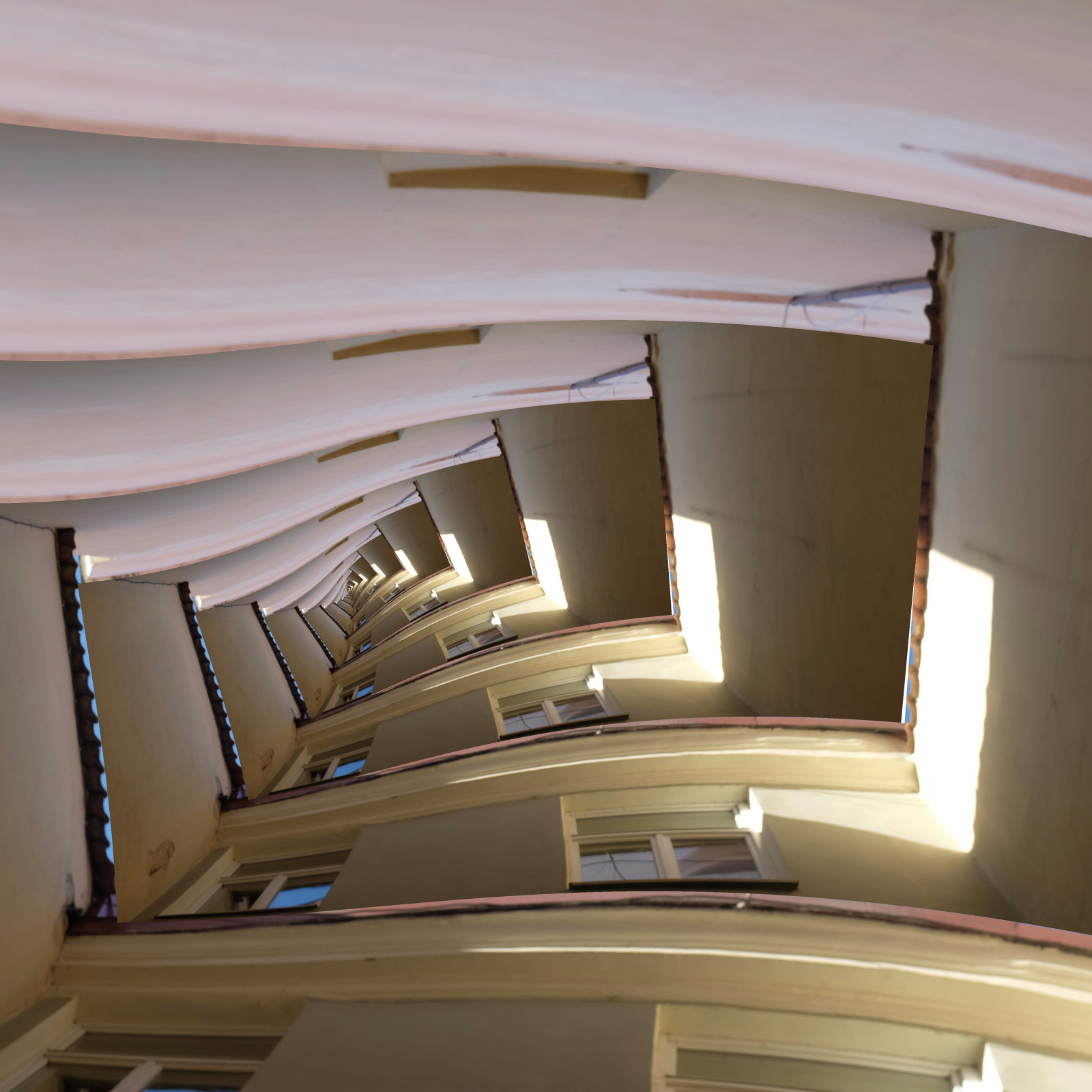
In this post, I’m going to explore how to implement the so-called “Droste effect.” The Droste effect is a name given to pictures that contain themselves, like an infinite series of nesting dolls. The conventional Droste effect is interesting, but it was taken to new heights by M.C. Escher’s “Print Gallery.”

The Print Gallery has the peculiar quality that if you follow the gaze of the person in the lower right corner, into the picture he is looking at, and around the image clockwise you find that you have come back to where you started: looking at a figure, looking at a picture. In some sense, this is a “Droste” picture: the print gallery contains a picture of the city that the print gallery is located in, except “zooming in” is replaced by walking around the origin.

Mathematicians and artists in the Netherlands managed to reverse-engineer the picture, and determined a transformation that can take an ordinary Droste image to a twisted, Escher-like image. They published an article explaining how it works, but on first and second reading I will admit I could make neither head nor tails of it. If it makes more sense to you, the rest of this post is going to be mostly superfluous! If you want to play with an existing implementation, check out Photospiralysis, which works in the browser.

I wanted to understand how Escher’s Print Gallery effect actually worked, and implement it myself. Luckily, the incomparable Jos Leys has written a pretty straightforward explanation, with pictures & equations. Most of the following is going to be lifted directly from his article, except we’re going to implement it as we read along. I recommend you read his article first, or at least give it a skim.

The implementation will be as a GLSL fragment shader (aka pixel shader). These are fast, and if you stick to GLSL2.0, it will work happily in the browser and many other places. If you’ve never touched fragment shaders, it would help to at least glance over The Book of Shaders first. I am borrowing the author’s code framework for displaying live examples.

Jos Leys explains how the transformation goes forward from a square picture to a Droste picture. To work as a fragment shader, we’re going to invert the transformation. For each point in the Droste picture, we work out which point on the original picture maps to it, and color our pixel accordingly. Working in this mode gives a feel of “warping space” rather than warping the image directly.

We’ll begin the same: with an annulus, the area between two circles. I am eliding how the annulus is actually drawn, mostly because I’m not an expert shader writer and my code isn’t great. Read The Book of Shaders linked above if you want to learn more about drawing shapes in GLSL.

Don’t forget that these examples are editable: adjust parameters and comment code out to see how it changes the result.

We are going to think of the annulus as actually sitting in the complex plane. We can perform complex arithmetic on our pixels! If you’re unfamiliar with complex numbers, it suffices for our purposes to know that complex numbers have two “coordinates” (real and imaginary) and points in the complex plane can be represented as a single number: $(x,y)$ in the ordinary plane can be thought of as $x+yi$, a complex number. In GLSL, complex numbers are stored identically to a point in the plane: a vec2.

You can perform arithmetic on complex numbers in similar ways to ordinary numbers. Addition, multiplication, and exponentiation all have equivalents in the complex plane. Most important for us is the complex exponent and its inverse, the complex logarithm.

$z \rightarrow \log(z)$ has the property that it transforms complex numbers within $r$ units of the origin into a strip $2 \pi$ high and $\log(r)$ wide.

$z \rightarrow \log(\frac{z}{r1})$ takes the annulus to a similar strip: points inside the annulus are transformed into points within a strip $2 \pi$ high and $\log(\frac{r2}{r1})$ wide.

The inverse transformation is $z \rightarrow e^{z} \cdot r1$. Transforming our coordinate system this way before we draw the circle will have the same effect as drawing the circle and then transforming it forward by the $\log$ transformation.

And we obtain the strip we were looking for. But wait, it’s infinitely tall! What’s going on? The complex $\log$ is a multi-valued function: it maps the annulus to an infinite number of strips, all stacked up. It’s defined as the inverse of the exponential function, and the exponential function actually takes points inside the infinitely tall ribbon to the annulus over and over again.

So, now we’re in what I call $\exp$-space. The rules are a bit different here. Just looking at the strip we have, left and right correspond to “in-out” in ordinary space; up and down correspond to rotating around the origin. This is the property that will generate the telescoping copies we want! We tile the ribbon horizontally in $\exp$-space using the modulo function:

This looks like the wrong order, but since we’re actually building an inverse function, later transformations need to be applied above earlier ones. Let’s use $\log$ to leave $\exp$-space and see what our infinite tiling achieved. Even though above I said that the complex logarithm was a multi-valued function, we can define a version that acts like an ordinary function and returns a single value (the principal value).

Wow! We’re well on our way. Each strip is transformed into another annulus, one nested inside the other. We can zoom in or out as much as we want, and there will always be another nesting annulus. We are sure of this because of the infinite tiling in $\exp$-space.

By rotating and scaling the strips in $\exp$-space, we can create the spiral effect we are looking for. The transformation code here is just an inversion of the Jos Ley’s transformation in his step (2): $z \rightarrow \frac{z}{e^{\theta i} \cdot cos(\theta)}$.

$a+bi$ and $a+(b+2\pi)i$ are transformed to the same point under the complex logarithm. After this rotation and scale, the top-right corner of each strip is exactly $2\pi$ above the bottom-left. After the logarithmic transformation, the upper right corner of each strip will coincide with the bottom-left corner of the previous. The inner circle and outer circle will connect! The result is a smooth spiral.

Try commenting out the tiling in the following example. You’ll see how the rotation in $\exp$ space has “torn” the annulus along the positive real axis. The tear is (I believe) a visual branch cut. The tiling repairs the tear by bringing in an infinite number of sheets that extend across all of the branches of the complex logarithm. I’ve been attempting to teach myself just enough complex analysis to understand this part, so my explanation may not in fact make any sense. At least, with some playing around, you can see how it works geometrically.

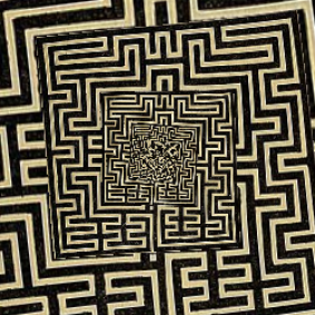
Now we have a Droste effect put together, we can abstract it out to a function. Rather than drawing an annulus, we’re going to draw a simple pattern to show what the effect does to more arbitrary shapes. Notice that with a small r1 it begins to resemble the Print Gallery, except the twist is going in the other direction.

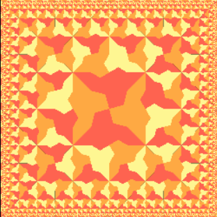
Only now does the most important property of this transformation become apparent: it is conformal, which means it preserves angles locally. Where two lines met at right angles before the transformation, they still do after being Drostified. This means that pictures transformed this way are very likely to remain recognizable.

In the next post(s), I’ll explore how to handle Drostifying a square. I’ll also show how to generalize the effect by adjusting how much it twists, how many arms the spiral has, and more.

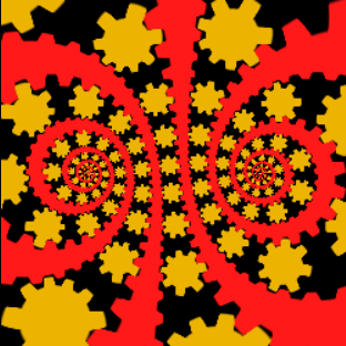
As a reward for making it all the way to the end, here’s an example of what you can do with the Droste effect! On the left is the original animation, and on the right the Droste transformation has been applied.