Drawing fractal Droste images
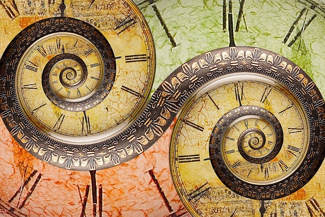
When I was researching Droste images for a previous post, I occasionally came across versions which depicted multiple spirals, rather than the ordinary single spiral, like this one by David Pearson. This led me down a rabbit hole to understand what is actually going on in these images, and to see what I could make with the effect.
This is going to be a longer post, so feel free to scroll to the end to see the final fractal results. Spoiler alert: Mandelbrots.
As with my previous posts, the embedded examples are all live shader code, and will automatically update as you edit them. They might not work correctly on all computers; your browser must support WebGL without too many bugs.
To begin with, I’m going to talk about complex functions. Complex functions take a complex number as input and return another. It’s a bit tricky to visualize them, since between the two-dimensional range and two-dimensional domain, the result is four-dimensional. A common method for visualizing these functions is domain coloring.
The idea behind domain coloring is that you draw a picture of a complex function $f: \mathbb{ C } \mapsto \mathbb{ C }$ by coloring the domain and pulling those colors back by $f$. In other words you color $z$ the same as $f(z)$ is colored. The particular method I’m using is called a phase portrait, borrowed from Elias Wegert. It colors the domain by the phase, or the angle it makes with the positive real axis. For more information, his article on the subject is a must-read.
In the example above, I’m just drawing the domain with no complex function at all (or, if you like, the identity $f: z \mapsto z$). Notice that it’s very obvious where $0$ is, because the colors all “bunch up” around it. We’ll see a similar effect near the zeros of a more complicated function. Here is the phase portrait for $f: z \mapsto z / (z^2 + z + 1)$.
Something funny’s happening. There’s three zero-like regions, but the two on the left are different- if you follow the hues around in a circle, they are cycling the “wrong way”. They’re not zeros at all, but poles: the center of these regions is where $f$ goes to infinity. You can’t explain this easily without invoking the Riemann sphere, which is much less intimidating than it sounds.

Imagine that the complex plane is actually sitting in 3D space. If you place a sphere at the origin, you can stereographically project points on the plane (complex numbers) to the sphere and back again, by casting a ray out from the top of the sphere. The lower hemisphere is identified with the unit disk, while the northern upper is identified with the entire rest of the plane. This is the Riemann sphere. An ant that lives on the complex plane that starts at the origin, can march outwards and the further it goes, the further its twin on the sphere approaches the north pole. If we map our domain coloring to the Riemann sphere, the colors get “gathered together” at the top of the sphere, which is why they gather together around infinities as well.
On the sphere above, I’ve drawn a circle with radius $0.5$ to help orient us; it gets projected to the lower hemisphere. Wave your mouse cursor over the sphere to tip it up and down. The sphere is raymarched based on this code.
The next step is to note that a logarithmic spiral projected back onto the sphere is a loxodrome, or rhumb line. This is caused by the logarithmic spiral being also “equiangular”: at every point, if you draw a circle centered at the origin that goes through it, the tangent will always make the same angle with the circle. Under stereographic projection, that circle becomes a parallel. Luckily for us, it’s easy to generate one: a circle transformed by the droste effect is a logarithmic spiral. Let’s superimpose that on our domain coloring to see how it looks on the sphere.
The awesome thing here is that we have a smooth spiral that is (roughly speaking) symmetrical across the equator. If we leave this spiral in our domain coloring, we will get smooth spirals around the zeros and poles of the phase portrait. So far as I know, this is actually a new (or at least rarely used) way to visualize complex functions.
The big reveal here is, we’re not just working with logarithmic spirals. We’re working with the droste effect! So we can draw a complicated Droste image in the domain and it will behave in a similar way.
To draw the two-spiral effect that we saw in the original image, we transform the domain with a Möbius transformation $z \mapsto \frac{z-1}{z+1}$. Notice that this function has one zero at $z=1$ (the numerator is $0$) and a pole at $z=-1$ (the denominator is $0$). This is equivalent, as you can see, to tipping the Riemann sphere sideways by 90 degrees.
The result applied to our droste domain is more or less similar to the two-spiraled effect that we wanted to emulate in the first place.
From here, there’s any number of complex functions we could play with. Elias Wegert’s phase plot gallery gives a sense of the variety. I decided to draw a Mandelbrot / Julia set.
The simplest method to draw a Mandelbrot image is to iterate each point $z_0$ through the Mandelbrot function $m(z) = z^2 + z_0$ until it escapes (or doesn’t) and then coloring the pixel accordingly, giving up at some large number of iterations. Instead, we’re just going to apply the function $n$ times and ignore whether it’s escaping or not, to produce a function $M_n$. Here I draw $M_3$:
This produces an interesting result, but I found that applying the Mobius transformation I used before produces a more satisfying picture. This is because the $M_n$ function (in the limit) maps the interior of the Mandelbrot set onto the unit disk. Placing the top and bottom of the loxodrome on the unit circle means that the “interesting” parts of the domain get mapped to somewhere near the boundary.
Instead of tipping the whole domain, you can just shift the top pole to the unit circle and leave the zero alone with $z \mapsto \frac{z}{z+1}$. It produces better results for slightly higher values of $n$, because it’s drawing spirals between the boundary of the Mandelbrot and the zeros in the interior. Try experimenting with this here, and above to see what it does to the Riemann sphere.
And finally, here’s an interactive animation of the Julia set; it alters the parameter $c$ based on mouse movement. This looks a bit like an orbit trap, but it’s not: orbit traps take the point with the smallest magnitude, I’m just taking the final one.
There is also a version listing the full source code rather than the abbreviated code displayed so far.
 Infinite Regression: Many Pictures From One Function
 Implementing the Droste effect in WebGL
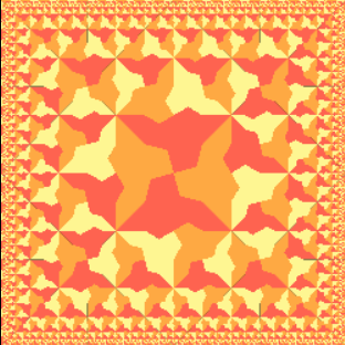 Building Escher's Square Limit in Pixels